Matières
Niveaux
| Fonctions | Règles de base | Règles transformées | ||
|---|---|---|---|---|
| Degré 0 | ||y=b|| | |||
| Degré 1 | ||y=x|| | Forme fonctionnelle | Forme symétrique | Forme générale |
||y=ax+b|||a| : taux de variation |b| : ordonnée à l'origine||a=\dfrac{y_2-y_1}{x_2-x_1}|| | ||\dfrac{x}{a}+\dfrac{y}{b}=1|||a| : abscisse à l'origine |b| : ordonnée à l'origine | ||Ax+By+C=0|| | ||
| |\Rightarrow| symétrique||\begin{align}a_s&=\dfrac{-b_f}{a_f}\\b_s&=b_f\end{align}|| | |\Rightarrow| fonctionnelle||\begin{align}a_f&=\dfrac{-b_s}{a_s}\\b_f&=b_s\end{align}|| | |\Rightarrow| fonctionnelle||\begin{align}a_f&=\dfrac{-A}{B}\\b_f&=\dfrac{-C}{B}\end{align}|| | ||
|\Rightarrow| générale Dénominateur commun et mettre tout du même côté | |\Rightarrow| générale Dénominateur commun et mettre tout du même côté | |\Rightarrow| symétrique||\begin{align}a_s&=\dfrac{-C}{A}\\\\b_s&=\dfrac{-C}{B}\end{align}|| | ||
| Degré 2 | ||y=x^2|| | Forme générale | Forme canonique | Forme factorisée |
| ||y=ax^2+bx+c|| | ||\begin{align}y&=\text{a}\big(b(x-h)\big)^2+k\\y&=\text{a }b^2(x-h)^2+k\\y&=a(x-h)^2+k\end{align}|| | Deux zéros||y=a(x-z_1)(x-z_2)||Un seul zéro||y=a(x-z_1)^2|| | ||
| Nombre de zéros||\sqrt{b^2-4ac}|| | Nombre de zéros||\sqrt{\dfrac{-k}{a}}|| | Nombre de zéros Directement accessible dans l'écriture de l'équation (voir la case au-dessus). Fait à noter : s'il n'y a aucun zéro, il est impossible d'utiliser cette forme. | ||
| Valeur des zéros||\dfrac{-b\pm\sqrt{b^2-4ac}}{2a}|| | Valeur des zéros||h\pm\sqrt{\dfrac{-k}{a}}|| | Valeur des zéros |z_1| et |z_2| | ||
| Valeur absolue | ||y=\vert x\vert|| | Forme canonique | ||
| ||\begin{align}y&=\text{a }\vert b(x-h)\vert+k\\y&=\text{a }\vert b\vert\times\vert x-h\vert+k\\y&=a\ \vert x-h\vert+k\end{align}|| | ||||
| Racine carrée | ||y=\sqrt{x}|| | Forme canonique | ||
| ||\begin{align}y&=\text{a}\sqrt{b(x-h)}+k\\[3pt]y&=\text{a}\sqrt b\sqrt{\pm(x-h)}+k\\[3pt]y&=a\sqrt{\pm(x-h)}+k\end{align}|| | ||||
| Partie entière | ||y=[x]|| | Forme canonique | ||
| ||y=a\big[b\,(x-h)\big]+k|| | ||||
| Fonctions | Règles de base | Règles transformées | Définitions et lois |
|---|---|---|---|
| Exponentielle | ||f(x)=c^x|| | ||f(x)=a(c)^{b(x-h)}+k|| | ||\begin{align}a^0&=1\\[3pt]a^1&=a\\[3pt]a^{-m}&=\dfrac{1}{a^m}\\[3pt]a^{^{\frac{\large{m}}{\large{n}}}}&=\sqrt[\large{n}]{a^m}\\[3pt]a^m=a^n&\!\!\ \Leftrightarrow\ m=n\\[3pt]a^ma^n&=a^{m+n}\\[3pt]\dfrac{a^m}{a^n}&=a^{m-n}\\[3pt](ab)^m&=a^mb^m\\[3pt](a^m)^{^{\Large{n}}}&=a^{mn}\\[3pt]\left(\dfrac{a}{b}\right)^m&=\dfrac{a^m}{b^m}\\[3pt]\sqrt[\large{n}]{ab}&=\sqrt[\large{n}]{a}\ \sqrt[\large{n}]{b}\\[3pt]\sqrt[\large{n}]{\dfrac{a}{b}}&=\dfrac{\sqrt[\large{n}]{a}}{\sqrt[\large{n}]{b}}\end{align}|| |
| Logarithme | ||f(x)=\log_cx|| | ||f(x)=a\log_c(b(x-h))+k|| | ||\begin{align}\log_c1&=0\\[3pt]\log_cc&=1\\[3pt]c^{\log_{\large{c}}m}&=m\\[3pt]\log_cc^m&=m\\[3pt]\log_cm=\log_cn\ &\Leftrightarrow\ m=n\\[3pt]\log_c(mn)&=\log_cm+\log_cn\\[3pt]\log_c\left(\dfrac{m}{n}\right)&=\log_cm-\log_cn\\[3pt]\log_c(m^n)&=n\log_cm\\[3pt]\log_cm&=\dfrac{\log_sm}{\log_sc}\end{align}|| |
| L'une est la réciproque de l'autre||x=c^y\ \Longleftrightarrow\ y=\log_cx|| | |||
| Fonctions | Règles de base | Règles transformées | Particularités |
|---|---|---|---|
| Sinus | ||f(x)=\sin x|| | ||f(x)=a\sin\big(b(x-h)\big)+k|| | ||\begin{align}\vert a\vert&=\dfrac{\max-\min}{2}\\[3pt]\vert b \vert&=\dfrac{2\pi}{\text{période}}\\[3pt]\text{Ima}f&=[k-a,k+a]\end{align}||Zéros : Une infinité de la forme |(x_1+nP)| et |(x_2+nP)| où |x_1| et |x_2| sont des zéros consécutifs, |n\in\mathbb{Z}| et |P| est la période. |
| Cosinus | ||f(x)=\cos x|| | ||f(x)=a\cos\big(b(x-h)\big)+k|| | |
| Tangente | ||f(x)=\tan x|| | ||f(x)=a\tan\big(b(x-h)\big)+k|| | ||\vert b\vert=\dfrac{\pi}{\text{période}}\\[3pt]\text{Dom}\ f=\mathbb{R}\backslash\left\{\left(h+\dfrac{P}{2}\right)+nP\right\}||où |n\in\mathbb{Z}| et |P| est la période. Zéros : Une infinité de la forme |x_1+nP| où |x_1| est un zéro, |n\in \mathbb{Z}| et |P| est la période. |
| Arc sinus | ||f(x)=\arcsin(x)||ou||f(x)=\sin^{-1}(x)|| | ||f(x)=a\arcsin\big(b(x-h)\big)+k|| | |
| Arc cosinus | ||f(x)=\arccos(x)||ou||f(x)=\cos^{-1}(x)|| | ||f(x)=a\arccos\big(b(x-h)\big)+k|| | |
| Arc tangente | ||f(x)=\arctan(x)||ou||f(x)=\tan^{-1}(x)|| | ||f(x)=a\arctan\big(b(x-h)\big)+k|| | |
| Identités de base | |||||
|---|---|---|---|---|---|
| ||\sin^2\theta+\cos^2\theta=1|| | ||1+\tan^2\theta=sec^2\theta|| | ||1+\text{cotan}^2\theta=\text{cosec}^2\theta|| | |||
| Autres identités | |||||
| ||\begin{align}\sin(a+b)&=\sin a\cos b+\cos a\sin b\\[3pt]\sin(a-b)&=\sin a\cos b-\cos a\sin b\\[3pt]\cos(a+b)&=\cos a\cos b-\sin a\sin b\\[3pt]\cos(a-b)&=\cos a\cos b+\sin a\sin b\\[3pt]\tan(a+b)&=\dfrac{\tan a+\tan b}{1-\tan a\tan b}\\[3pt]\tan(a-b)&=\dfrac{\tan a-\tan b}{1+\tan a\tan b}\end{align}|| | ||\begin{align}\sin2x&=2\sin x\cos x\\[3pt]\cos2x&=1-2\sin^2x\\[3pt]\tan2x&=\dfrac{2}{\text{cotan}x-\tan x}\\[3pt]\sin(-\theta)&=-\sin\theta\\[3pt]\cos(-\theta)&=\cos\theta\\[3pt]\sin\left(\theta+\dfrac{\pi}{2}\right)&=\cos\theta\\[3pt]\cos\left(\theta+\dfrac{\pi}{2}\right)&=-\sin\theta\end{align}|| | ||||
| Les théorèmes dans le cercle |
|---|
Les théorèmes en lien avec les rayons, les diamètres, les cordes et les arcs :
Les théorèmes en lien avec les angles :
Les théorèmes en lien avec les sécantes et les tangentes au cercle :
|
| Rapports trigonométriques (triangles rectangles) | Lois trigonométriques (triangles quelconques) | |
|---|---|---|
| ||\sin A=\dfrac{\text{Opposé}}{\text{Hypoténuse}}|| | ||\text{cosec }A=\dfrac{1}{\sin A}=\dfrac{\text{Hypoténuse}}{\text{Opposé}}|| | ||\dfrac{\sin A}{a}=\dfrac{\sin B}{b}=\dfrac{\sin C}{c}|| |
| ||\cos A=\dfrac{\text{Adjacent}}{\text{Hypoténuse}}|| | ||\text{sec }A=\dfrac{1}{\cos A}=\dfrac{\text{Hypoténuse}}{\text{Adjacent}}|| | ||\begin{align}a^2&=b^2+c^2-2bc\cos A\\[3pt]b^2&=a^2+c^2-2ac\cos B\\[3pt]c^2&=a^2+b^2-2ab\cos C\end{align}|| |
| ||\tan A=\dfrac{\text{Opposé}}{\text{Adjacent}}|| | ||\text{cotan}A=\dfrac{1}{\tan A}=\dfrac{\text{Adjacent}}{\text{Opposé}}|| | |
| Composantes |\boldsymbol{(a,b)}| d'un vecteur | |||
|---|---|---|---|
| ||a=\Vert \overrightarrow{u}\Vert \cos \theta|| ||b=\Vert \overrightarrow{u}\Vert \sin \theta|| | Soit le vecteur |\overrightarrow{AB}| avec |A(x_1, y_1)| et |B(x_2, y_2)| Alors, les composantes sont : ||a=x_2-x_1\\b=y_2-y_1|| | ||
| Norme d'un vecteur | |||
| Soit le vecteur |\overrightarrow{u}=(a,b)| Alors, la norme est : ||\Vert\overrightarrow{v}\Vert=\sqrt{a^2+b^2}|| | Soit le vecteur |\overrightarrow{AB}| avec |A(x_1, y_1)| et |B(x_2, y_2)| Alors, la norme est : ||\Vert\overrightarrow{AB}\Vert=\sqrt{(x_2-x_1)^2+(y_2-y_1)^2}|| | ||
| Orientation d'un vecteur | |||
| |\theta=\tan^{-1}\left(\displaystyle\frac{b}{a}\right)| |
| ||
| Somme de deux vecteurs | |||
| Soit |\overrightarrow{u}=(a,b)| et |\overrightarrow{v}=(c,d)| Alors, |\overrightarrow{u}+\overrightarrow{v}=(a+c,b+d)| | |\Vert \overrightarrow{u}+\overrightarrow{v}\Vert=\Vert \overrightarrow{u}\Vert+\Vert \overrightarrow{v}\Vert-2\Vert \overrightarrow{u}\Vert\ \Vert \overrightarrow{v}\Vert\ \cos\theta| où |\theta =\ \Large{\mid} \normalsize 180^o - \mid \theta_\overrightarrow{u}-\theta_\overrightarrow{v}\mid \Large{\mid}| | ||
| Soustraction de deux vecteurs | |||
| Soit |\overrightarrow{u}=(a,b)| et |\overrightarrow{v}=(c,d)| Alors, |\overrightarrow{u}-\overrightarrow{v}=(a-c,b-d)| | |\Vert \overrightarrow{u}+\overrightarrow{v}\Vert=\Vert \overrightarrow{u}\Vert+\Vert \overrightarrow{v}\Vert-2\Vert \overrightarrow{u}\Vert\ \Vert \overrightarrow{v}\Vert\ \cos\theta| où |\theta=\mid \theta_\overrightarrow{u}-\theta_\overrightarrow{v}\mid| si |\mid \theta_\overrightarrow{u}-\theta_\overrightarrow{v}\mid<180^o| et |\theta = 180^o - \mid \theta_\overrightarrow{u}-\theta_\overrightarrow{v}\mid| sinon | ||
| Multiplication par un scalaire | |||
| Soit |k| un scalaire et |\overrightarrow{u}=(a,b)| Alors, |k\overrightarrow{u}=(ka,kb)| ||\begin{align}\Vert k \overrightarrow{u} \Vert &= k \times \Vert\overrightarrow{u}\Vert \\ \theta_{k \overrightarrow{u}} &= \theta_{\overrightarrow{u}} \end{align}|| | |||
| Produit scalaire | |||
| Si le produit scalaire est de |0|, alors les vecteurs sont perpendiculaires. | |||
| À l'aide des composantes Soit |\overrightarrow{u}=(a,b)| et |\overrightarrow{v}=(c,d)| Alors, |\overrightarrow{u}\cdot \overrightarrow{v}=ac+bd| | À l'aide de la norme et de l'orientation |\overrightarrow{u}\cdot \overrightarrow{v}=\Vert\overrightarrow{u}\Vert\times \Vert\overrightarrow{v}\Vert\times \cos\theta| | ||
| Propriétés de l'addition de deux vecteurs | |||
| 1) La somme de deux vecteurs est un vecteur. | |||
| 2) Commutativité | |\overrightarrow{u}+\overrightarrow{v}=\overrightarrow{v}+\overrightarrow{u}| | ||
| 3) Associativité | |(\overrightarrow{u} + \overrightarrow{v}) + \overrightarrow{w} = \overrightarrow{u} + (\overrightarrow{v} + \overrightarrow{w})| | ||
| 4) Existence d'un élément neutre | |\overrightarrow{u}+\overrightarrow{0}=\overrightarrow{0}+\overrightarrow{u}=\overrightarrow{u}| | ||
| 5) Existence d'opposés | |\overrightarrow{u}+(-\overrightarrow{u})=-\overrightarrow{u}+\overrightarrow{u}=\overrightarrow{0}| | ||
| Propriétés de la multiplication par un scalaire | |||
| 1) Le produit d'un vecteur par un scalaire est toujours un vecteur. | |||
| 2) Associativité | |k_1(k_2\overrightarrow{u})=(k_1k_2)\overrightarrow{u}| | ||
| 3) Existence d'un élément neutre | |1\times \overrightarrow{u}=\overrightarrow{u}\times 1=\overrightarrow{u}| | ||
| 4) Distributivité sur l'addition de vecteurs | |k(\overrightarrow{u}+\overrightarrow{v})=k\overrightarrow{u}+k\overrightarrow{v}| | ||
| 5) Distributivité sur l'addition de scalaires | |(k_1+k_2)\overrightarrow{u}=k_1\overrightarrow{u}+k_2\overrightarrow{v}| | ||
| Propriétés du produit scalaire | |||
| 1) Commutativité | |\overrightarrow{u}\cdot \overrightarrow{v}=\overrightarrow{v}\cdot \overrightarrow{u}| | ||
| 2) Associativité des scalaires | |k_1\overrightarrow{u}\cdot k_2\overrightarrow{v}=k_1k_2(\overrightarrow{u}\cdot\overrightarrow{v})| | ||
| 3) Distributivité sur une somme vectorielle | |\overrightarrow{u}\cdot(\overrightarrow{v}+\overrightarrow{w})=(\overrightarrow{u}\cdot\overrightarrow{v})+(\overrightarrow{u}\cdot\overrightarrow{w})| | ||
| Concepts | Formules | |||||
|---|---|---|---|---|---|---|
| Accroissements | ||\begin{align}\Delta x&=x_2-x_1\\[3pt]\Delta y&=y_2-y_1\end{align}|| | |||||
| Distance entre deux points | ||d(A,B)=\sqrt{(x_2-x_1)^2+(y_2-y_1)^2}|| | |||||
| Coordonnées du point de partage | Rapport partie au tout | Rapport partie à partie | ||||
| ||\begin{align}x_p&=x_1+\dfrac{r}{s}(x_2-x_1)\\[3pt]y_p&=y_1+\dfrac{r}{s}(y_2-y_1)\end{align}|| | ||\begin{align}x_p&=x_1+\dfrac{r}{r+s}(x_2-x_1)\\[3pt]y_p&=y_1+\dfrac{r}{r+s}(y_2-y_1)\end{align}|| | |||||
| Coordonnées du point milieu | ||(x_m,y_m)=\left(\dfrac{x_1+x_2}{2},\dfrac{y_1+y_2}{2}\right)|| | |||||
| Pente d'une droite | ||a=\dfrac{\Delta y}{\Delta x}=\dfrac{y_2-y_1}{x_2-x_1}|| | |||||
| Comparaison de deux droites d'équations |y=ax+b| | Parallèles confondues | Parallèles disjointes | Perpendiculaires | |||
| ||\begin{align}a_1&=a_2\\[3pt]b_1&=b_2\end{align}|| | ||\begin{align}a_1&=a_2\\[3pt]b_1&\neq b_2\end{align}|| | ||a_1=-\dfrac{1}{a_2}|| | ||||
| Transformations | Règles | Réciproques |
|---|---|---|
| Translation | ||t_{(a,b)}:(x,y)\stackrel{t}{\mapsto}(x+a,y+b)|| | ||t^{-1}_{(a,b)}=t_{(-a,-b)}:(x,y)\stackrel{t}{\mapsto}(x-a,y-b)|| |
| Rotation | ||\begin{align}r_{(O,90^\circ)}&:(x,y)\stackrel{r}{\mapsto}(-y,x)\\[3pt]r_{(O,-270^\circ)}&:(x,y)\stackrel{r}{\mapsto}(-y,x)\\[3pt]r_{(O,180^\circ)}&:(x,y)\stackrel{r}{\mapsto}(-x,-y)\\[3pt]r_{(O,-90^\circ)}&:(x,y)\stackrel{r}{\mapsto}(y,-x)\\[3pt]r_{(O,270^\circ)}&:(x,y)\stackrel{r}{\mapsto}(y,-x)\end{align}|| | ||\begin{align}r^{-1}_{(O,90^\circ)}&=r_{(O,-90^\circ)}\\[3pt]r^{-1}_{(O,-270^\circ)}&=r_{(O,270^\circ)}\\[3pt]r^{-1}_{(O,180^\circ)}&=r_{(O,180^\circ)}\\[3pt]r^{-1}_{(O,-90^\circ)}&=r_{(O,90^\circ)}\\[3pt]r^{-1}_{(O,270^\circ)}&=r_{(O,-270^\circ)}\end{align}|| |
Réflexion (Symétrie) | ||\begin{align}s_x&:(x,y)\stackrel{s}{\mapsto}(x,-y)\\[3pt]s_y&:(x,y)\stackrel{s}{\mapsto}(-x,y)\\[3pt]s_{\small/}&:(x,y)\stackrel{s}{\mapsto}(y,x)\\[3pt]s_{\tiny\backslash}&:(x,y)\stackrel{s}{\mapsto}(-y,-x)\end{align}|| | ||\begin{align}s^{-1}_x&=s_x\\[3pt]s^{-1}_y&=s_y\\[3pt]s^{-1}_{\small/}&=s_{\small/}\\[3pt]s^{-1}_{\tiny\backslash}&=s_{\tiny\backslash}\end{align}|| |
| Homothétie | ||h_{(O,k)}:(x,y)\stackrel{h}{\mapsto}(kx,ky)|| | ||h^{-1}_{(O,k)}=h_{\left(\frac{1}{k},\frac{1}{k}\right)}:(x,y)\stackrel{h}{\mapsto}\left(\dfrac{x}{k},\dfrac{y}{k}\right)|| |
| Coniques | Équations canoniques | Paramètres |
|---|---|---|
Cercle Lieu géométrique de tous les points situés à égale distance du centre. | ||x^2+y^2=r^2|| ||(x-h)^2+(y-k)^2=r^2|| | |r:| rayon |(h,k):| Centre du cercle |
Ellipse Lieu géométrique de tous les points dont la somme des distances aux deux foyers est constante. | ||\dfrac{x^2}{a^2}+\dfrac{y^2}{b^2}=1|| ||\dfrac{(x-h)^2}{a^2}+\dfrac{(y-k)^2}{b^2}=1|| | ||\begin{align}a&=\dfrac{\text{Axe horizontale}}{2}\\b&=\dfrac{\text{Axe verticale}}{2}\end{align}|| |(h,k):| Centre de l'ellipse |
Hyperbole Lieu géométrique de tous les points dont la valeur absolue de la différence de la distance aux foyers est constante. | ||\dfrac{x^2}{a^2}-\dfrac{y^2}{b^2}=\pm1|| ||\dfrac{(x-h)^2}{a^2}-\dfrac{(y-k)^2}{b^2}=\pm1|| | Asymptotes : ||\begin{align}y&=\dfrac{b}{a}(x-h)+k\\y&=-\dfrac{b}{a}(x-h)+k\end{align}|| |(h,k):| Centre de l'hyperbole |
Parabole Lieu géométrique de tous les points situés à égale distance de la directrice et du foyer | ||(x-h)^2=4c(y-k)|| ||(y-k)^2=4c(x-h)|| | ||\vert c\vert :\dfrac{\text{Distance foyer-directrice}}{2}|| |(h,k):| Sommet de la parabole |
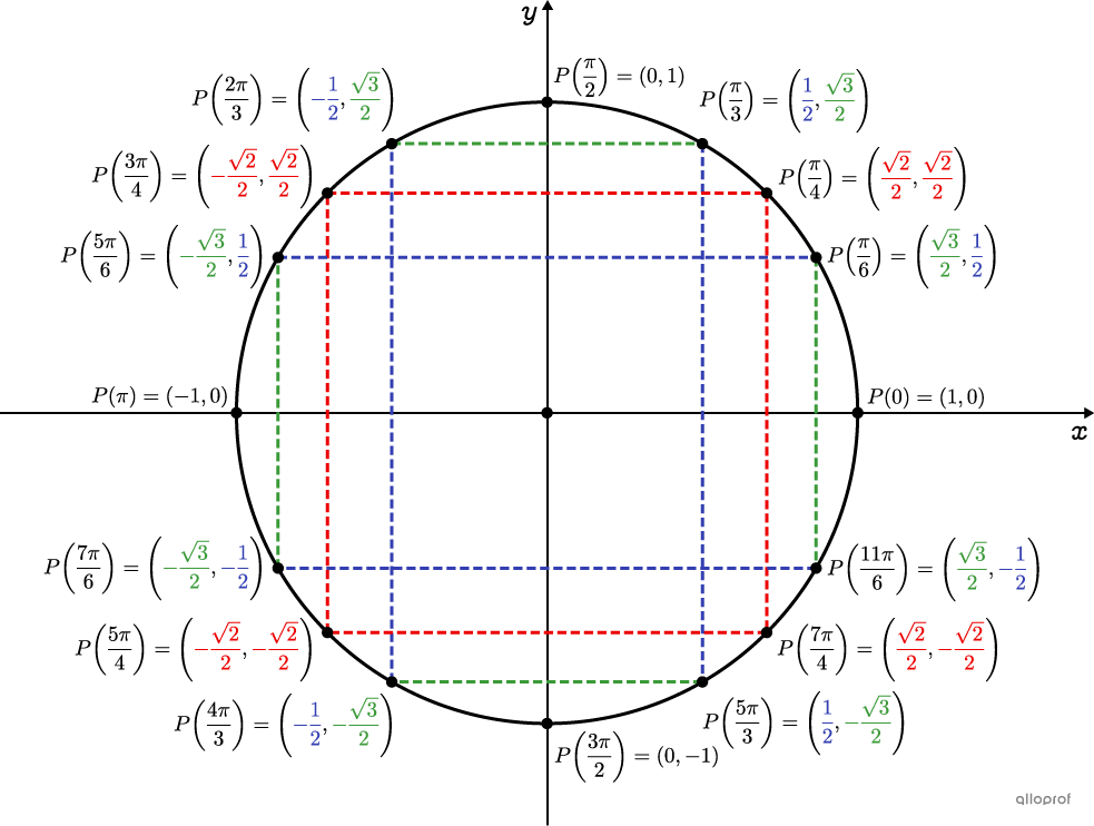
||P(\theta)=(\cos\theta,\sin\theta)||
| Concepts | Formules |
|---|---|
| Probabilité | ||\text{Probabilité}=\dfrac{\text{Nbr de cas favorables}}{\text{Nbr de cas possibles}}|| |
| Probabilité complémentaire | ||\mathbb{P}(A')=1-P(A)|| |
| Probabilité d'événements mutuellement exclusifs | ||\mathbb{P}(A\cup B)=\mathbb{P}(A)+\mathbb{P}(B)|| |
| Probabilité d'événements non mutuellement exclusifs | ||\mathbb{P}(A\cup B)=\mathbb{P}(A)+\mathbb{P}(B)-\mathbb{P}(A\cap B)|| |
| Probabilité conditionnelle | ||\mathbb{P}(B\mid A)=\mathbb{P}_A(B)=\dfrac{\mathbb{P}(B\cap A)}{\mathbb{P}(A)}|| |
| Espérance de gain | ||\mathbb{E}[\text{Gain}]=\text{Probabilité de gagner}\times\text{Gain net}+\text{Probabilité de perdre}\times\text{Perte nette}|| |
| Espérance mathématique | ||\mathbb{E[X]}=x_1\mathbb{P}(x_1)+x_2\mathbb{P}(x_2)+\ldots+x_n\mathbb{P}(x_n)||où les résultats possibles de |X| sont les valeurs |x_1, \ldots, x_n.| |